JupyterLab beyond simple widgets: interactive Lorentzian fitting

What's interactive Lorentzian fitting?#

If you ever tried to fit the curves like the below with a set of Lorentzian functions

you will know the importance of a good initial guess of the parameters. If you don't know about it, the task here is to find the best $A_i$, $\mu_i$, $\sigma_i$ and $C$ with the given experimental data, where $\mu$ is the center of the peak, $\sigma$ is a parameter specifying the width, $A$ is a parameter specifying the amplitude, and $C$ is a constant background. Since there are so many parameters and the curve can be quite different with different sets of parameters, it's hard to do the fitting without a sensible initial guess.

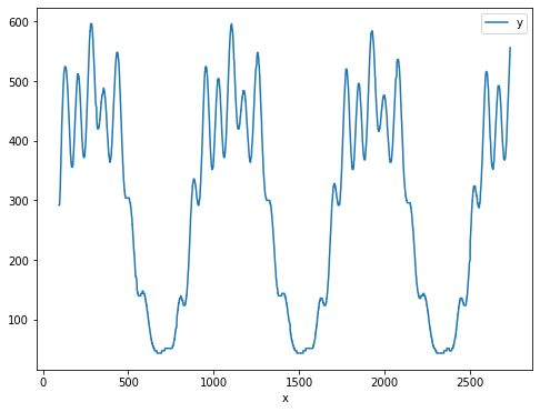
How to provide an initial guess? The most straightforward way is to guess reasonable $\sigma_0 = \sigma_i$, and the centers and heights of the peaks for $\mu_i$ and $A_i$. Other peaks can affect the center and height of the peak so it is a rough approximation, but enough in this case.

How to find the peaks, then? Of course, one can use the peak finding algorithm, but I had some bad times tuning the parameters of the peak finding function, and I don't like to hard-code the parameters. Instead, I'm going to provide the peaks manually. But again, no hard-code parameters, so copying all the coordinates into the code is not a desirable solution. I'd like to provide the peaks by interactively clicking on the plots.

Interactive JupyterLab plots#

Typical interactive Jupyter notebooks involve some buttons, sliders, and inputs, as the image above shows. But the examples haven't leveraged the power of Matplotlib. Matplotlib not only supports simple widgets like the sliders but also supports mouse clicks and many more events.

In this example, the button is provided by IPython, and the mouse events are handled by Matplotlib via ipympl. ipympl enables the interactive features of Matplotlib in Jupyter by passing the events to a live Python kernel.

ipympl is easy to install:

pip install ipympl
sh

And to enable it, just use %matplotlib ipympl magic in the notebook.

Click and update#

The basic example of handling mouse events is to add a scatter point on mouse clicks.

def click_and_update(figname):
    plt.close(figname)  # close the figure when rerun the cell
    fig = plt.figure(figname)
    ax = fig.subplots()
    points = []
    scatter_plot = ax.scatter([], [], marker="x")

    def onclick(event):
        if event.button == 1:  # LEFT
            points.append([event.xdata, event.ydata])
        xdata, ydata = zip(*points)
        scatter_plot.set_offsets(np.c_[xdata, ydata])
        fig.canvas.draw_idle()

    fig.canvas.mpl_connect("button_press_event", onclick)
    plt.show()

click_and_update("click_example")
python

In the onclick function, we first add the point to a list called points, and then update the scatter with set_offsets, and finally update the canvas with fig.canvas.draw_idle. We then connect the handler onclick with the button_press_event event. The final result should look like this:

The exceptions raised and lines printed in the on_click handler will not show up in the notebook. Instead, you can find the detailed logs in the log panel. If you can't find the button for the log panel in the status line, you can choose "View -> Activate Command Palette" in the menu and select "Show Log Console" to bring it up.

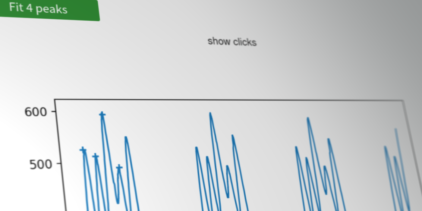
Click on the peaks and save them#

With the basic knowledge of Matplotlib event handling in JupyterLab, we can now start building the blocks for interactive fitting. The first step is to click on the peaks and save them.

def fit_data_peaks(data_file: Path, name: str):
    df = read_table(data_file)
    peak_file = PWD / "peaks" / f"{name}.json"
    result_file = PWD / "results" / f"{name}.json"

    plt.close(name)
    fig = plt.figure(name)
    ax = fig.subplots()
    ax.plot(df.x, df.y, label="Data")

    peak_scatter = None

    if not result_file.exists():
        if peak_file.exists():
            peaks = json.loads(peak_file.read_text())
            peak_scatter = ax.scatter(*zip(*peaks), marker="+")
        else:
            print("Peak file not found")
            peaks = []
            peak_scatter = ax.scatter([], [], marker="+")

        action_button = widgets.Button(
            description=f"Fit {len(peaks)} peaks", button_style="success"
        )

    def onclick(event):
        if event.button == 1:  # LEFT
            peaks.append([event.xdata, event.ydata])
        elif event.button == 3:  # RIGHT
            idmin = np.linalg.norm(
                np.array(peaks) - np.array([event.xdata, event.ydata]), axis=-1
            ).argmin()
            peaks.pop(idmin)
        else:
            return
        action_button.description = f"Fit {len(peaks)} peaks"
        xdata, ydata = zip(*peaks)
        peak_scatter.set_offsets(np.c_[xdata, ydata])
        fig.canvas.draw_idle()

    def do_fit(_):
        peak_file.write_text(json.dumps(peaks, indent=2))
        print("To be implemented")

    if result_file.exists():
        print("Plot the results. To be implemented.")
    else:
        fig.canvas.mpl_connect("button_press_event", onclick)
        action_button.on_click(do_fit)
        display(action_button)

    plt.show()
python

Here we define a function called fit_data_peaks. It first calls the read_table function which parses the data and returns a DataFrame with two columns, x and y. Then the data is plotted. Next, if the results haven't been stored, we go to the peak-clicking mode (the final else clause), where the on_click function handles most of the logic, which is similar to the previous example. One additional functionality is that when right-clicked, the peak point nearest to the cursor is removed, which can be quite useful. When the button is clicked, we are supposed to the curve fitting and save the results, but in this example, we just save the clicked peaks.

Fitting the curve#

I use the lmfit module for curve fitting, and use the uncertainties module for easy calculating the uncertainties.

from lmfit.model import load_modelresult, save_modelresult
from lmfit.models import ConstantModel, LinearModel, LorentzianModel
from lmfit.parameter import Parameters
python

    def do_fit(event):
        del event  # unused
        action_button.disabled = True
        peak_file.write_text(json.dumps(peaks, indent=2))
        gmodel = ConstantModel()
        for i in range(len(peaks)):
            gmodel += LorentzianModel(prefix=f"p{i}_")
        params = gmodel.make_params(c=0)
        init_sigma = 30
        for i, peak in enumerate(peaks):
            params[f"p{i}_center"].value = peak[0]
            params[f"p{i}_amplitude"].value = peak[1] * np.pi * init_sigma
            params[f"p{i}_sigma"].value = init_sigma
        fit_result = gmodel.fit(df.y, params, x=df.x)

        results[name] = fit_result

        save_modelresult(fit_result, result_file)

        plot_fit(fit_result)
python

In the do_fit function, a model is created according to the number of peaks and is fitted against the data using the fit method. Then the result is saved to a global variable results and to the result_file on the disk. Finally, it calls the plot_fit function to update the figure:

    def plot_fit(fit_result):
        if peak_scatter is not None:
            peak_scatter.remove()
        ax.plot(df.x, fit_result.best_fit, label="Fit")
        ax.legend()
        fig.canvas.draw_idle()
        fig.savefig(f"{name}.pdf")
python

It removes the peaks, plots the best fit provided by lmfit, updates the plot, and saves it to a PDF file.

Assemble them all#

You can find the codes at https://github.com/AllanChain/jlab-demo-interactive-fitting